1) a machine, which works reproducible
2) an exchange of qualities Qi with the machine, which are additive and deterministic
then the generalized first law means:
After a cycle of the machine the in- and effluxes
by W.D. Bauer ©, released 7.12.99, corrected 16.10.01, 06.03.02
1. Introduction
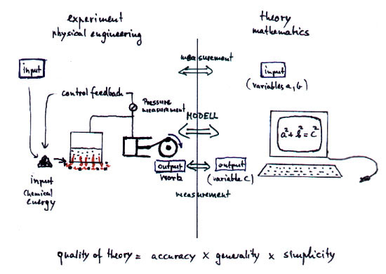
The essence of physics consists in the
mapping of real processes to theoretical mathematical models which should
show quantitatively the same features as found in reality. By defining
a physical measurement the variables in the theory are connected to the
physical reality. If the concerning variables of the theory coincide quantitatively
with the real measurements then we say the theory is correct, comp. fig.1.
Acc. to Newton physics is obliged to the
principle of "hypotheses non fingo", i.e. the implementation of physically
(or psychologically) motivated principles as mathematical constraints of
a theory should be avoided because this entrains a loss of generality and
the danger of arising inconsistencies. Nevermind, sometimes it is done
for tentative purposes, and sometimes this strategy even seems to
yield correct predictions. However, if such heuristically motivated constraints
cannot not be founded in a more general framework with time they survive
sometimes as "natural laws" for centuries because their preliminary heuristic
character is forgotten. They are vulgarized, overgeneralized, are combined
with economic interests and exert a considerable suggestive blocking pressure
on learning people.
"Natural laws" are not made by god but
by a man fitting the mapping of a mathematical theory to the experimental
reality using the term "natural law" as power amplifier for selling his
products and opinions . In reality any physical description is a compromise
between what we can see and what we want to see. And what we want to see
is determined by our social, economic, moral, religious and instinct motivated
prepolarisation which sets up our projections on that what we regard to
be the reality.
Due to such psychologically motivated
reasons misinterpretations oftenly apply especially to the fundamental
laws of physics like the first and second law. Therefore, we start our
article with very simple and banal mathematical ideas.
2. The generalized first law
2.1 Definition of a machine
We define a machine as a coherent volume
of space which exchanges one or more different qualities of quantities
with its environment (for instance mass, energy, angular momentum). The
volume of the machine (or the system border) can change as well. We demand
that the volume change and all exchange processes with environment can
be done periodically. We may or may not know what happens in the inner
of the machine. A simple scetch of a machine can be found in fig. 2. It
is clear that this definition extends not only to conventional machines
but to many physical processes as well, comp.[1,2]
2.2 The generalized first law
Physical processes are described normally
by differential equations. These can have relaxing, exploding or periodic
solutions. Otherwise, strange attractors or complete chaotic solutions
are possible. It is clear that a machine has to be able to work periodically
or -if we use a physical term- reproducible which means that the machine
process can be done periodically.
The coordinate of the exchanging qualities
has to be localized uniquely, i.e. in- or outside of the machine. This
means: the qualities are deterministic, i.e. uniquely defined in space
und time. The quantities can cross the border between the machine and environment.
With these concepts in mind we can formulate "our" generalized first law
Proposition:
We have
1) a machine, which works reproducible
2) an exchange of qualities Qi
with the machine, which are additive and deterministic
then the generalized first law means:
After a cycle of the machine the in- and
effluxes ![]() kQi
of the qualities Qi are zero
kQi
of the qualities Qi are zero

It is clear that a first law balance holds
generally only after a cycle is performed completely. Sometimes special
cases exist where the balance is fulfilled even from point to point of
a cycle but it does not hold generally if only a part of the cycle is proceeded.
An example for this is liquid water under 4 degree Celsius. If we take
off heat from it by cooling it down it expands and performs work. In sum
we get heat dQ and work dW by doing this process from A to B. The energy
balance dQ +dW =0 is fulfilled only after a complete cycle is proceeded
and the substance comes back to the initial starting point of the cycle.
After many cycles the impression appears
that the quantities are conserved because the mean of the total balance
is conserved in the mean if time goes to infinity.
In order to apply the first law correctly
we have to find out the range of validity of the above assumptions for
each qualitity Qi. It is clear that the proposition can not
cover quantum mechanically defined quantities because these are deterministic
only for limit cases. Furthermore, it is critical to apply it to irreversible
non-reproducible processes, because it is hardly possible to prove anything
under irreproducible conditions.
If concreticized the qualities Qi
can be energy, charge, mass, momentum and angular momentum. The applicability
and the consequences of the above proposition will be discussed for each
of these qualities in the next sections.
2.3. The first law applied for the quality
of energy
In classical physics the quality energy
E is defined generally by the equation


Examples:
1) Conservative systems
If we make concrete x and f with
All these examples seem to look quite trivial,
however if we change the meaning of the variables in examples of figures
4 we can easily find analog systems which appear to be perpetuum mobiles
of first kind, comp. tab.2 showing these analogies. For instance, if we
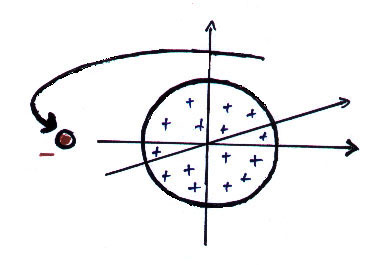
postulate a "strange" magnetic material coupling to a conservative magnetic
field then we can get running a magnetizable bowl on a circular track in
a magnetic field as shown in [3]. Here, acc. to the theory field energy
tapped is changed into work even if no "influx of magnetic energy" can
be detected from outside. Similarly, if we have (electric or magnetic)
capacitive material properties, which change parametrically in time, analogous
"overunity" effects are principally possible as well.[3]
In sum, we can conclude: Regardless, whether
energy in- or effluxes of a machine can be found experimentally or not,
a balance hold for every system under description. The "first law" is used
as a mathematical tool to calculate and to describe cycles: This means,
all machines including perpetuum mobiles of first kind fulfill the first
law per definition !
2.4 The first law applied for the quality
of mass
It is quite trivial that mass is an additive
quantity. It should be mentioned that -similarly for energy- this does
not hold for relativistic cases because then mass and energy cannot considered
separately. In this article such problems are not followed.
2.5 The first law applied for the quality
of charge
As well as mass charge is an additive
quantity and this hold even for the theory of relativity.
2.6 The first law applied for the quality
of momentum
Momentum is regarded as a conserved quantity
in the common sense of any physicist. However, critical examination shows
that it is appropriate to be more careful with this assumption. Generally,
momentum is not conserved for any system, whose Lagrangian is dependent
not only from a velocity coordinate but from a space coordinate as well.
Momentum conservation means always a special case of the equation of motion,
i.e.


2.7 The first law applied for the quality
of angular momentum
It is clear that analogous considerations
like that of the last section should be possible for angular momentum.
Consequently, it should exist an angular moment balance, an angular moment
potential for cyclic processes for periodic machines. However, the author
did not find balance equations of angular momentum in literature at first
sight. The cause of that may be that the standard definition of angular
momentum is not appropriate for a many particle system. The standard definition
of angular momentum is

3. A cycle with fluids in a field
3.1 Previous works
The idea that cycles binary mixtures in fields may violate the second
law was due to B. van Platen who became known as the inventor of adsorption
refrigerator[5]. A. Serogodsky made measurement on a similar cycle and
claimed to have measured such violations. Calculations with a modern equation
of state without fields did not confirm any claim of both [6,7].
These claims were tested out using two possible axiomatizations of thermodynamics.
The first axiomatization was based on the conventional Sears-Kestin version
of the second law which forbids per dogma any equation of state which give
such "strange"solutions. The other "axiomatization" was based on the extremum
principle of the potentials. The second possibility is only apparent but
not really an axiomatization of thermodynamics because it can be motivated
by a derivation of thermodynamics from mechanics [8]. It has the advantage
that it reduces the number of hypotheses. No additional "physical axiom"
like second law based on experience or overgeneralization (dependent from
your personal point of view) is necessary. The alternative axiomatization
derives the second law as a consequence of the mathematics of the system.
It allows the second law to reverse if fields are present as shown in [9].
Acc. to [6,7], both axiomatizations yield no second law violation for calculation
of a van Platen or Serogodsky cycle using a equation of state (EOS).
Therefore, in order to test out the van Platen claim completely it
is necessary to include the dependence from the field whose influence can
be significantly in the neighborhood of critical points. The idea
is near to use space-dependent thermodynamics including fields to test
out the equation of state behavior in fields as proposed indirectly already
in van Platen's patent.
A formal similar problem (but more simple 2-variable system independent
from any space coordinate) has been discussed recently by the author. This
model of a polymer solution system describes phase transitions in an electric
field. It is confirmed qualitatively in parts by experiments[11]. Consequent
application of this model predicts overunity behavior due to "irreversibilites
in the other direction" which are possible if one accepts the our interpretation
of second law[7].
By applying analogous considerations to other potential fields it is
possible to enlarge the number of possible candidates for second law violations.
In tab. 2 we give an overview of some possible fields which allow such
cycles. In appendix 3 the second variation of the least action functional
is derived for gravitation and centrifugal fields indicating the possibility
2nd law violating cycles.
3.2 General formalism of space dependent equilibrium thermodynamics including potential fields
3.2.1 General thermodynamic theory
It is well known that any static thermodynamic
material property can be described generally by a potential like inner
energy U(S,V,ni) or G(P,T,ni) chosen acc. to the
problem under question.
If fields are taken into account, the
thermodynamic equations become dependent from the (here one-dimensional)
space coordinate r additionally . Then, the ansatz of inner energy U*
in field can be written [8]

 := gravitational potential and dV:=A.dr. We denote P* as the
global total pressure (a fictive value without any physical observable
relevance), which is constant and characterizes mathematically the global
coupling over the whole volume. Similarly µi*
is the global total chemical potential. This general formalism makes thermodynamics
dependent from the space coordinate r of the field, it includes not only
the description of barometric and hydrostatic pressure phenomena (if P*
0
[10]), but furthermore allows to calculate density and concentration profiles
of fluids in fields. The formulas are surely not new and coincide with
known derivations[12].
:= gravitational potential and dV:=A.dr. We denote P* as the
global total pressure (a fictive value without any physical observable
relevance), which is constant and characterizes mathematically the global
coupling over the whole volume. Similarly µi*
is the global total chemical potential. This general formalism makes thermodynamics
dependent from the space coordinate r of the field, it includes not only
the description of barometric and hydrostatic pressure phenomena (if P*
0
[10]), but furthermore allows to calculate density and concentration profiles
of fluids in fields. The formulas are surely not new and coincide with
known derivations[12].
3.2.2 Phase equilibrium with field
Acc. to the standard Gibbs the variation
the inner energy at a interface of two phases


3.2.3 Conclusions
In general, if a field is present, pressure
gradients are generated which induce as well concentration gradients in
the volume. Therefore, phase equilibria differ from point to point along
the field direction. At each point r of the volume, however, the local
equilibrium state and the rate constants can be determined acc. to usual
thermodynamics without field, if P(r),T, and xi(r) are known.
Due to the global coupling in the volume, the equilibria shift in sum relatively
to the uniform state without field, especially if
1) the molecular weights of the components
are high
2) high pressure differences arise in
the fluid due to a high field which induces high differences in the activities
of the components as well, or
3) the local different barometric pressures
in the system are in the neighbourhood of a critical point and even slight
variation of parameters of P generated by the field can produce big variations
in activities and densities of the fluid.
Furthermore, phase equilibria can depend
from the shape of the vessel due to global coupling of the particle number
over the whole volume. The dependence of the pressure profile depends from
the form of the vessel i.e. the hydrostatic paradoxon fails to exist generally
for multicomponent systems.
3.3 The computation of thermodynamic equilibrium of a mixture in a field with a equation of state
In the following we will describe how the general theory of the last section can be made concrete by a numerical solution of a phase equilibrium. We will describe subsequently the different program modules (or numeric functions) which - if built together - allow to calculate the phase equilibrium in a field.
3.3.1 The Bender equation of state-
the subroutine EQOFSTATE
In order to get a good accuracy in our
calculation we take a modern generalized Bender equation of state[14] which
allows to calculate analytically for all thermodynamical properties and
which can be programmed economically using the Horner sceme[14,15]. The
equation has the form


3.3.2 Calculation of phase equilibrium
- the subroutine NEWTONGAUSS
In order to calculate the phase equilibrium
the equations of the Gibbs fundamental system have to be solved. The first
equation equals pressure in vapor and liquid

3.3.3 The inverted equation of state
V(P,T,xi) - The subroutine V_PTX
The Bender equation of state is formulated
analytically in the form P(v,T,xi) with v, T and xi
as independent variables. For some purposes however (as we will see below)
it is appropriate to have the same equation of state (EOS) in the form
V(P,T,xi). If we want to know the thermodynamical state in dependence
from P0, T and xi, the inversion is done numerically
by solving the equation
3.3.4 The thermodynamic state dependent
from P and fi - the subroutine VX_PF
Because the inverted EOS is needed for
the least square algorithm a subroutine has been to evaluate the EOS values
dependent from P,T and xi. With T constant and skipped here
such a set consists of equations for


3.3.5 The thermodynamic statedependent
from P and µi - the subroutine VTX_PMu
In order to calculate the compartment
array of a fluid under a field it is appropriate to have the set of constitutive
equations dependent from P and µi. Such a set consists
of equations for


3.3.6 The volume array calculation in
an arbitrary potential field- the subroutine VOLUME (Footnote)
If a field is applied pressures and chemical
potentials differ from point to point. The subroutine VOLUME calculates
the profiles of pressure, concentration and chemical potentials along the
space coordinate of the known field if in one point of the volume P and
xi are known. Our program calculates only one-dimensional profiles
in a tubular housing,
Generalization to more dimensions and
other forms of housings would be easily possible but is not done here.
For calculation the whole volume is divided into a array of m equal subvolumes
dV(rj ) (at same potential) at the space coordinate rj.
At one point rref called reference point we assume
to know the pressure P(rref) and the concentration xiref
.
Then, all other points in the volume are interconnected to their neighbor
compartment by the equations for (hydrostatic) pressure using g(rj-1)=-dV(rj-1)/dr

For concrete programming the formula µi=µi0(p+,T)+
RT
ln(fi /p+) + Mi .V(r) has to be applied.
The subroutine sums up as well the total
number Ni of each particle in the total volume because it is
needed in the next subroutine. Therefore, the algorithm proceeds as follows
:
1) Define the number M of volume
array cell, i.e. the partition of the volume .
2) Give pressure P0,
temperature T0 and concentrations xi at one point
rref called the reference point
3) Using the subroutine V_PX
invert numerically the equation of state at rref and
calculate v
4) Initialize the particle numbers
Ni=0
5) FROM volume array cell J=1 TO
M
6) Determine
all interesting thermodynamic data at rj using EQOFSTATE,
especially µi and dni(rj),
i.e. the number of particles of each sort i in this subsection dV(rj)
of V
7) Ni=Ni+dNi(rj
) Add up the particle number in the compartment to find the total number
of the array
8) Determine
P and µi in the next adjacent volume section dVj+1
acc. to equations (27) + (28)
9) Invert
numerically the equation of state at rj+1 and calculate v,T,xi
using the subroutine VTX_PMu
10) NEXT J
11) Give out all calculated values
3.3.7 Volume array calculation at conserved
particle numbers - the subroutine N_PX
Because the total particle number is conserved
in the most problems, the volume array in the field has to determined under
the constraint Ni0=consti. Acc. to the
last section 3.3.6 the total particle numbers Ni in the volume
is calculated in the subroutine VOLUME . This numbers can be regarded
as numerical functions of the starting values Pref and xiref
in
VOLUME , i.e.

3.3.8 Fitting generalized Bender equation
to empirical mixture data -the subroutine LEASTSQUARES
Because only few published unreliable
fit parameter exist for mixtures calculated using the Bender equation,
the fit constants must be calculated from empirical data. Therefore, a
known least square fit algorithm [19] and [20] was implemented in
a subroutine LEASTSQUARES. This sub-routine fits the parameter kij, ![]() and
and ![]() to empirical
values. The input of this routine contains the starting values of the fit
constants, experimental values, fixed parameters like material constants,
allowed errors and switches used for economical programming. The output
of this routine consists of the results of the iteration, i.e. the fit
constants and furthermore the least squares sum values and errors documenting
the performance of the iteration. For a critical discussion of the fit
method and its results click here
.
to empirical
values. The input of this routine contains the starting values of the fit
constants, experimental values, fixed parameters like material constants,
allowed errors and switches used for economical programming. The output
of this routine consists of the results of the iteration, i.e. the fit
constants and furthermore the least squares sum values and errors documenting
the performance of the iteration. For a critical discussion of the fit
method and its results click here
.
4. Results
We used Argon-Methan data [21] to test
our algorithm. The choice of this system was due to wrong expectation disproved
in the course of the investigations and was continued then as lab rat for
study. For practical purposes under environment conditions, mixtures of
Nitrogen, Argon, SF4, SF6 as superheated component
and Propane, Butane, CO, CO2 as condensable component are possible.
(We omit here the classical refrigerants.)
First, we calculated appropriate fit constants
to the data using the least square routine. For results click here
! With these model data we calculated the rotator cycle. We choosed as
field free initial state a mixture with a molar ratio of Argon of 56%,
55 bar and 170 K. This is very near in the neighborhood of the critical
point in the gaseous ara of the phase diagram, comp. fig.8 . The rotator
cycle is shown in fig.9. The closed volume of the mixture is set under
rotation. At 4000 RPM the total volume is split unsymmetrically into two
halves by a tap. The split point is chosen arbitrarily at the point where
the specific volume in the field equals about the specific volume without
field. Then, both volumes are decelerated again to the field free situation.
Fig. 10a)- c) shows the pressure, concentration and specific molar volume
profiles versus radius in the centrifugal field each during acceleration
(upper diagrams) and deceleration (lower diagrams). Fig. 11 shows the work
diagram of the cycle calculated from the diagrams of Fig.10a)-c)
using a tabel calculation program.
5.Discussion
The orientation of the isothermal cycle indicates a mechanical energy loss. This can be seen if we write down the definition of work.
![]()
Appendix 1: The Poynting energy conservation reduced to a energy conversion formula
The Poynting formula is written


Appendix 2: Momentum conservation of a many particle system with internal central forces
Proposition:
Inner forces do not contribute to the
total momentum of a many particle system if they are central forces between
the particles which can be derived from a potential.
Proof:
We assume that the force between the molecules
i and j is a potential function dependent only from distance, i.e. V(ri-rj).
The Hamiltonian for the whole system including inner forces is

If we regard the total force on the whole system we get

Appendix 3: Second variation of gravitational and centrifugal fields
A) Centrifugal field
For thermodynamic potentials including
centrifugal fields holds


B) Gravitational field
For thermodynamic potentials including
force fields like gravitation holds


Appendix 4: The degrees of freedom of a multicomponent mixture in a potential field
In order to calculate a phase equilibrium we consider a tubular volume filled with fluid with n components in a field V(r) with the coordinate r. As an approximation the volume is divided into m compartments for calculation purposes. In each compartment the equation of state is fulfilled locally with defined values P(v(rj),xi(rj), T(rj)) and µi(v(rj),xi(rj), T(rj)), comp. fig.A4.1(last pic) .
Numbers of equations:
1) The next equation shows that the pressure
equation is linearly dependent from the chemical potential equations.

Therefore, between two adjacent compartments
exist each n equations. It is recommended to take only the equations of
chemical potential for calculation purposes in order to avoid integrals
in the algorithm. Therefore, n.(m-1) equations (32) and (33) exist between
the m compartments, indicated by the double arrows in equ. 47 !
2) Additionally we have n equations of
mass conservation (see equs. 35), i.e.
Number of variables:
Because temperature is constant over the
volume we have n.m unknown variables v(m) and xi(m)
over the volume.
Therefore, because the numbers of variables
is equal to the numbers of equations, the system is determined completely.
Appendix
5: Calculation of the thermodynamic state of a real fluid with a Bender
equation of state
Bibliography:
[1] W.H. Müller, W. Muschik J.Non-Equilib.
Thermodyn. Vol.8 (1983) p. 29 - 46
Bilanzgleichungen offener mehrkomponentiger
Systeme I. Massen und Entropiebilanzen (in German)
[2] W. Muschik, W.H. Müller J. Non-Equilib.
Thermodyn. Vol.8 (1983) p. 47 - 66
Bilanzgleichungen offener mehrkomponentiger
Systeme II. Energie und Entropiebilanz (in German)
[3] W.D.Bauer at http://www.overunity-theory.de/magmotor/magmotor.htm
Do non-conservative potential perpetual
running machines exist
[4] F.Kuypers Klassische Mechanik 5.AuflageWiley-VCH
1997
[5] van Platen US patent 4.084.484 18.4.1978
[6] Bauer W.D., Muschik W. J. Non-Equilib.
Thermodyn. Vol.23, No.2,1998, p.141 -158
[7] Bauer W.D., Muschik W. Archives of
Thermodynamics Vol.19, No.3-4, 1998, p.59-83
[8] Bauer W.D. From mechanics to thermodynamics
http://www.overunity.com/2ndlaw/2ndlaw.htm
[9] Bauer W.D. Incompatibility of Planck's
Version of Second Law Regarding Mixtures in Fields http://www.overunity-theory.de/bauer/index.html
[10]V.Freise Chemische Thermodynamik BI
Taschenbuch 1973 (in German)
[11] D. Wirtz, G.G. Fuller Phys.Rev.Lett.71
(1993) 2236
[12] J.U. Keller Thermodynamik der irreversiblen
Prozesse, de Gruyter, Berlin, 1977 (in German)
[13] Bhattacharya K., Friesecke G., James
R.D.
Proc. Natl. Acad. Sci. USA Vol.96,pp.8332-8333
1999
The mathematics of microstructure and
the design of new materials
[14] Platzer, B.
Eine Generalisierung der Zustandsgleichung
von Bender zur Berechnung von
Stoffeigenschaften polarer und unpolarer
Fluide und deren Gemische
Dissertation Fachbereich Maschinenbau
Universität Kaiserslautern 1990 (in
German)
[15]Polt, A. Zur Beschreibung der thermodynamischen
Eigenschaften reiner Fluide mit
erweiterten BWR-Gleichungen Fachbereich
Maschinenbau Uni Kaiserslautern 1986/87
[16] Tsai F.-N., Shuy J.-H.
Prediction of High-Pressure Vapor-Liquid
Equilibria by the Corresponding-States Principle
Journal of the Chin. I. Ch. E., Vol.16,No.2,
198, p. 157-163
[17]Reid, R.C., Prausnitz, J.M., Poling,
B.E. The Properties of Gases and Liquids, McGraw-Hill, New York 1987
[18] Stephan K., Mayinger F. Thermodynamik
Bd.II
Springer Verlag Berlin, New York 1988
[19] Fletcher, R.
A modified Marquard Subroutine for Non-Linear
Least Squares
U.K.A.E.A. Research Group Atomic Energy
Research Establishment
(AERE) - R.6799, Harwell 1971
[20] Ahrendts J., Baehr H.J.
Die Anwendung nichtlinearer Regressionsverfahren
bei der Aufstellung thermodynamischer
Zustandsgleichungen (in German)
Forsch. Ing.Wes. 45 1979 no.2 p.51-56
[21] Christiansen L.J., Fredenslund Aa..,
Mollerup J., Cryogenics July 1973 p.405-413
[22] P. Debye, K. J. Kleboth
J. Chem.Phys.42 (1965) 3155
[23] Coats C. , Living energies - Viktor
Schauberger´s brilliant work
GATEWAY BOOKS 1996 The Hollies,Wellow,
Bath, BA2 8QJ, UK
in German: Naturenergien verstehen und
nutzen -Viktor Schaubergers geniale Entdeckungen
Omega-Verlag, Düsseldorf, 1999
Tables:
Table 1: different realizations of the
energy integral ![]() f dx
f dx
|
|
|
|
|
|
|
|
|
|
|
|
|
|
|
|
|
|
|
|
|
|
|
|
|
|
|
|
|
|
|
|
|
|
|
|
Table 2: different possible and postulated
realizations of non-conservative force fields
|
|
|
|
|
| windmill | angle | "wind" field energy | mechanical energy |
| "strange" iron ball
in magnetic field |
path x | magnetic field energy | mechanical energy |
| parametric changing inductivity | time t | magnetic field energy | electric current |
| parametric changing
capacitance |
time t | electric field energy | electric current |
Table 3: Overview of possible additional
thermodynamic variables with potential extremum behaviour
|
|
|
|
|
|
- H dM |
Maximum (if µ>0) |
|
|
- P dE |
Maximum (if |
|
|
- |
Maximum |
|
|
with ( F=m.g(r) ) - F dr |
Maximum |
Captions:


 |
 |